Supercharge Your Shallow ML Models With Hummingbird

Photo by
[Levi Jones](https://unsplash.com/@levidjones?utm_source=unsplash&utm_medium=referral&utm_content=creditCopyText)
on
[Unsplash](https://unsplash.com/s/photos/hummingbird?utm_source=unsplash&utm_medium=referral&utm_content=creditCopyText) — Photo by Levi Jones on Unsplash

Motivation

Since the most recent resurgence of deep learning in 2012, a lion's share of new ML libraries and frameworks have been created. The ones that have stood the test of time (PyTorch, Tensorflow, ONNX, etc) are backed by massive corporations, and likely aren't going away anytime soon.

This also presents a problem, however, as the deep learning community has diverged from popular traditional ML software libraries like scikit-learn, XGBoost, and LightGBM. When it comes time for companies to bring multiple models with different software and hardware assumptions into production, things get...hairy.

How do you keep ML inference code DRY when some models are tensor-based and others are vector-based?
How do you keep the inference runtime efficiency of your traditional models competitive, as GPU-based neural networks start to run circles around them?

In Search of A Uniform Model Serving Interface

I know, I know. Using microservices in Kubernetes can solve the design pattern issue to an extent by keeping things de-coupled...if that's even what you want?

But, I think that really just ignores the problem. What if you want to seamlessly deploy either an XGBoost regressor or fully-connected DNN as your service's main output? Sure, you could hot-swap the hardware your service launches onto. How about the code?

Are you going to ram in a dressed-up version of an if-else switch to use one software framework vs the other, depending on the model type?

Isn't XGBoost/LightGBM Fast Enough?

Well, for a lot of use cases, it is. However, there's still a huge gap between problems requiring neural nets and problems that can be sufficiently solved with more traditional models. For the more traditional models, don't you still want to be able to use the latest and greatest computational frameworks to power your model's predictions? This would allow you to scale your model up more before you need to resort to scaling it out via redundant instances.

Enter Hummingbird

Microsoft research has introduced hummingbird to bridge this gap between CPU-oriented models and tensor-oriented models. The library simply takes any of our already-trained traditional models and returns a version of that model built on tensor computations. Hummingbird aims to solve two core concerns with current ML applications:

Traditional and deep learning software libraries have different abstractions of their basic computational unit (vector vs tensor).
As a result of this difference, traditional ML libraries do not receive the same performance gains as hardware accelerators (read: GPUs) improve.

With Hummingbird, your ML pipelines will start to look cleaner. You'll know that, regardless of the algorithm, you end up with a model that creates its predictions via tensor computations. Not only that, these tensor computations will be run by the same deep learning framework of choice that your organization has likely already given allegiance to.

All of this from one function call. Not a bad deal in my book!

Let's see it in action.

Setup

Let's get this part out of the way. You know the drill.

      
        !pip install seaborn
      
        !pip install hummingbird_ml
      
        !pip install hummingbird-ml[extra]
      
        !pip install torch torchvision
      
        !pip install onnxruntime-gpu
      
        !pip install onnxmltools>=1.6.0

view raw hummingbird-deepnote_1.py hosted with ❤ by GitHub

      
        import torch
      
        import numpy as np
      
        import pandas as pd
      
        import matplotlib.pyplot as plt
      
        import seaborn as sns
      
        import mpl_toolkits
      
        from sklearn.datasets import make_classification
      
        from sklearn.model_selection import train_test_split
      
        from sklearn.ensemble import RandomForestRegressor
      
        from hummingbird.ml import convert
      
        print('GPU available: %s' % torch.cuda.is_available())
      
        %matplotlib inline

view raw hummingbird-deepnote_2.py hosted with ❤ by GitHub

Ensure Reproducibility

Let's control randomness in Numpy and PyTorch with the answer to everything in the universe.

      
        RND_SEED = 42
      
        np.random.seed(RND_SEED)
      
        torch.manual_seed = RND_SEED
      
        torch.backends.cudnn.deterministic = True
      
        torch.backends.cudnn.benchmark = False

view raw hummingbird-deepnote_3.py hosted with ❤ by GitHub

Conjure Some Data

Let's define a quick helper to quickly make some classification data, and create some data sets with it.

      
        def make_data(n_samples=1000):
      
            """
      
            Return some synthetic classification data from sklearn.datasets.
      
            @param int n_samples: number of samples the data set should have.
      
            @param int n_features: number of features the data set should have.
      
            @return tuple:
      
                [0]: numpy.ndarray data set of shape (n_samples, n_features)
      
                [1]: numpu.ndarray labels of shape (n_samples, )
      
            """
      
            X, y = make_classification(
      
                n_samples=int(n_samples), n_features=20,
      
                n_informative=8, n_redundant=2, n_repeated=0, n_classes=2, n_clusters_per_class=2,
      
                shuffle=True, random_state=42
      
            )
      
            return X.astype('|f4'), y

view raw hummingbird-deepnote_4.py hosted with ❤ by GitHub

      
        X_train, y_train = make_data(n_samples=1e3)
      
        X_test, y_test = make_data(n_samples=1e4)
      
        clf = RandomForestRegressor(n_estimators=250, max_depth=10)
      
        clf.fit(X_train, y_train)

view raw hummingbird-deepnote_5.py hosted with ❤ by GitHub

Thanks to Deepnote, I don't have to take up half of this notebook just printing out data shapes and distributions for you. These notebooks come with a feature-packed variable explorer which provides most of the basic EDA-style questions you will have about your data.

Check out the original version of this article to see how Deepnote automatically creates beautiful articles from their Jupyter-style notebooks.

Bring in the Bird

Now, the one-liner to get your model transformed into tensor computations via Hummingbird is convert(clf, 'pytorch').

That's it. That's Hummingbird.

Just to make our comparisons even easier, let's make a quick method on top of that to automatically move it to a GPU when it's available. As some final added sugar, we'll take in a flag that forces keeping the model on CPU, should the need arise. Keep in mind though, the single call to convert() is the only interface you need to have with Hummingbird; it does all of its magic under the hood of that single function call. Once you get the model returned to you, you call predict() on it like any other traditional pythonic ML model.

      
        def compile_pytorch(model, force_cpu=False):
      
            """
      
            Use Hummingbird to compile a PyTorch model, moving it to a GPU if available.
      
            @param Model model: trained ML model which has a predict() method for inference.
      
            @param bool force_cpu: whether to keep the model on CPU, regardless of the presence of a GPU.
      
            @return Model: augmented ML model, which uses tensor computations to perform inference
      
            """
      
            model = convert(clf, 'pytorch', extra_config={"tree_implementation":"gemm"})
      
            if torch.cuda.is_available() and not force_cpu:
      
                print('Moving model to GPU')
      
                model.to('cuda')
      
            else:
      
                print('Keeping model on CPU')
      
            return model

view raw hummingbird-deepnote_6.py hosted with ❤ by GitHub

      
        print('Creating CPU Hummingbird model\n\t', end='')
      
        clf_cpu = compile_pytorch(clf, force_cpu=True)
      
        print('Creating GPU Hummingbird model\n\t', end='')
      
        clf_gpu = compile_pytorch(clf)

view raw hummingbird-deepnote_7.py hosted with ❤ by GitHub

Get Your Watches Out, It's Time to Time

Alright, it's time to benchmark! Don't worry about a flurry of imports or method wrappers. Let's keep it simple here with the %%timeit magic command. This magic command will automatically run the code in the cell multiple times, reporting out the mean and standard deviation of the runtime samples. First, we'll time the sklearn model as-is. Then, we'll see how the Hummingbird on-CPU and on-GPU models compare.

      
        %%timeit
      
        clf.predict(X_test)

view raw hummingbird-deepnote_8.py hosted with ❤ by GitHub

      
        %%timeit
      
        clf_cpu.predict(X_test)

view raw hummingbird-deepnote_9.py hosted with ❤ by GitHub

Original: 136 ms ± 1.59 ms per loopHummingbird CPU: 1.81 s ± 16.1 ms per loop

Source: Giphy

Yikes!

Well...that was unexpected. There are no two ways about this one: Hummingbird might run slower on CPU for certain data sets. This can even be seen by some of their current example notebooks in the Hummingbird Github repo. Also, I did mention that the runtime is slower on certain data sets with intention, as it does outperform for others.

That being said, this side effect shouldn't have anyone running for the door --- remember the library's goal! The main reason for converting a model to tensor computations is to leverage hardware that excels in that area.

Spoiler alert: I'm talking about GPUs! This Deepnote notebook comes powered by an NVIDIA T4 Tensor Core GPU. Let's see how the model runs on that.

      
        %%timeit
      
        clf_gpu.predict(X_test)

view raw hummingbird-deepnote_10.py hosted with ❤ by GitHub

Original: 136 ms ± 1.59 ms per loopHummingbird CPU: 1.81 s ± 16.1 ms per loopHummingbird GPU: 36.6 ms ± 65.8 µs per loop

There we go! Now, we not only have a 73% mean speedup over the original, but also an order of magnitude tighter variance. The original standard deviation of runtime is 1.1% of its mean, and the GPU runtime's standard deviation is 0.18%!

Source: Giphy

Ensuring Quality with Speed

Hold in your excitement for now, though. Your model could have the fastest runtime in the world; if it doesn't maintain its accuracy through the conversion, it could be utterly useless. Let's see how the predictions compare between the original model and both transformed models. For this, we turn to one of my favorite visualization libraries, seaborn.

      
        # get predictions from the models for the same data
      
        y_pred = clf.predict(X_test)
      
        y_pred_cpu = clf_cpu.predict(X_test)
      
        y_pred_gpu = clf_gpu.predict(X_test)
      
        def plot_distributions(data_label_pairs, title='Score Distribution(s)'):
      
            """
      
            Plot the distribution of a list of prediction vectors.
      
            @param List data_label_pairs:
      
            """
      
            plt.figure(figsize=(12, 6))
      
            for data, label in data_label_pairs:
      
                sns.distplot(data, hist=False, label=label)
      
            plt.legend()
      
            plt.xlabel('x')
      
            plt.ylabel('P(x)')
      
            _ = plt.title(title)
      
        plot_distributions(
      
            [
      
                [y_pred_cpu - y_pred, 'Δ predictions for HB CPU'],
      
                [y_pred_gpu - y_pred, 'Δ predictions for HB GPU']
      
            ],
      
            title='Checking the Predictive Distribution Divergence'
      
        )

view raw hummingbird-deepnote_11.py hosted with ❤ by GitHub

Distribution of prediction differences between original and Hummingbird models

Interesting...

Not bad at all. The distribution of the deltas for the CPU-based model is rather symmetric around zero with a 3σ (note the axis scale) around 1e-7. The distribution of the deltas for the GPU-based model has a similarly small deviation, but show a non-zero bias and a skew! This is certainly interesting behavior that piques the curious mind, but it remains a small detail for all but the most precision-sensitive models.

The jury is in: Hummingbird delivers precision alongside the speedup 👍.

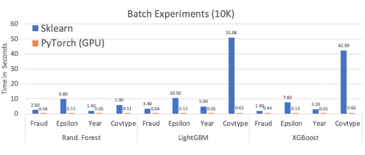
Check out the comparisons below from some of Microsoft's larger-scale comparisons. 🚀

Source:
[Microsoft Research](https://azuredata.microsoft.com/articles/ebd95ec0-1eae-44a3-90f5-c11f5c916d15) — Source: Microsoft Research

The Cherry On Top

Oh, and by the way, you also automatically plug into all of the future computational optimizations that come from the thousands of people employed to work on these mega-frameworks. As support for the less popular frameworks dies off (trust me, it eventually happens), you will sit comfortably, knowing that every one of your models run on well-supported, tensor-based inference frameworks.

After all, we're in the business of data science, not runtime optimization. It feels good to leverage the big guys to get the job done in that area, freeing us up to focus on our core competencies.

Conclusion

As with a lot of other recent moves by Microsoft Research, I'm excited about Hummingbird. This is a great step towards consolidation in the rapidly diverging ML space, and some order from chaos is always a good thing. I'm sure the runtime hiccups of their CPU-based inferencing will be smoothed out over time while ensuring continued advantages on the GPU. As their updates get made, we're just a few clicks away from a GPU-enabled Deepnote notebook ready to test their claims!

Dive Into Hummingbird

Use Hummingbird With Deepnote